|
[first posted: 23 December 1995, revised 10 July 2000, 30 January 2001, and 12 September 2003]
 CorTech
Training, Red Wing, MN CorTech
Training, Red Wing, MN
Weibull Trending Toolkit (WTT)
Courses I, II and
III are presented to students of engineering everywhere, at
all career stages. They contain elements useful for development
of Safety Critical (SC) Systems for many types of containment structures.
Many containments are pressure vessels. When a fluid is contained
under pressure, it is important that it be designed to leak
before it breaks. Corrosion pits can cause leaks. They can
also serve as initiation sites for crack growth. When a
growing crack penetrates a container wall, the crack growth
mechanism must not convert from a slow growth to a fast or catastrophic
fracture mode. Spend time searching topics such as safety critical
systems, artificial neural networks for SC systems.
INTRODUCTION
This course examines historic data sets containing depths of
pits measured after sets of ferrous alloy specimens had been
exposed to corrosion environments for extended periods of
time. Ferrous alloys require corrosion protection. Depending
on the type of alloy and application, the protection can be
in the form of zinc galvanizing, cadmium or other plating, or
an inhibitive coating or lining system. In critical
applications, such as aircraft structures, periodic
inspections are performed to ensure protection system
integrity. A surficial irregularity such as a carbon or
carbide particle, or minute scratch can cause a local spot to
be galvanically noble with respect to the base alloy. A
corrosion pit can form at the irregularity.
COURSE
FOCUS
Corrosion consultant, test engineer, and inspector roles in
pipeline testing are central. Main points of lessons and
numerical exercises are based on instructor's experience in
reviewing and analyzing pit depth data sets. The Weibull
Trending Toolkit and QBasic programs are used extensively.
Auditors are expected to read lessons and follow instructor's
guidelines in repeating numerical exercises.
COURSE OUTLINE
-
Task 1
Review
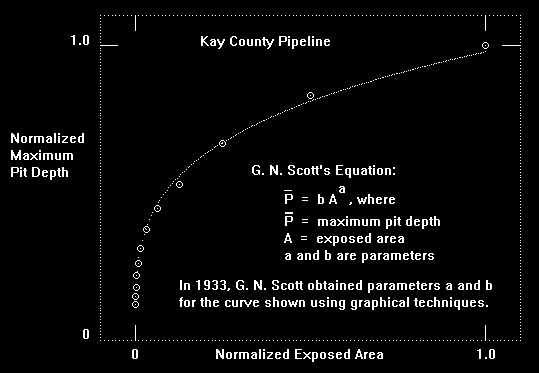
G. N. Scott's 1933 analysis
of Kay County pipeline
maximum pit depth versus exposed area and analyze the
data by linear regression.
- Task 2
Analyze
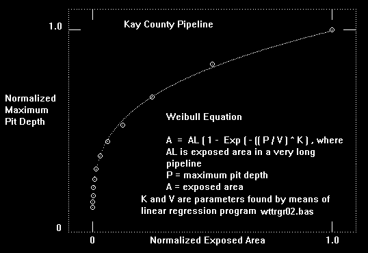
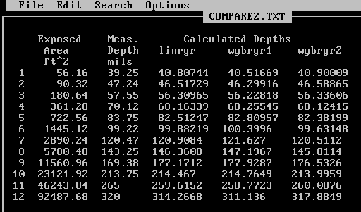
the Kay County data by means of two Weibull curve fitting
relations and compare with Scott's results.
Task 3
Apply
Weibull relations to G. N. Scott's Mt. Auburn and
Council Hill data and to Mahoning and
Almeda-Lynchburg data obtained by other
investigators.
Task 4
Review
G. G. Eldredge's 1957 interpretation of Bessemer
steel data obtained by K. H. Logan (1945) and analyze
the data by Weibull analyses.
Task 5
Analyze
K. H. Logan's 1945 wrought iron specimen data and
compare with Bessemer steel specimen results.
Task 6
Review
P. M. Aziz's 1956 experimental procedures and data
for Al alloy specimens immersed in Kingston tap
water.
Task 7
Interpret
Aziz's pitting depth frequency distributions by
Weibull analysis.
Task 8
Interpret
Aziz's Alcan 55S-T maximum pit depth data for 9 or 10
specimens at each of six exposure times.
Task 9
Generalize
interpretations of Aziz's data to obtain a relation
in terms of exposed area, maximum pit depth, and
exposure time.
e-mail from Bob Heidersbach concerning G. N. Scott:
Glenn
Thanks to you and your website, I know about Gordon Scott's early work. I am proof reading a book I've written and needed a slightly better reference than the one you have on the problem #1 web page. I found this information, which seems to be from something at the U of Michigan. The URL is as the bottom.
Thanks again for remaining a valuable contributor to rusty knowledge.
Bob Heidersbach
Cape Canaveral, Florida
Scott, G. N. The Use and Behavior of Protective Coatings on Underground
Pipes. Am. Petroleum Inst. Bull. I, 1928, pp. 78-93.
186. - API Pipe Coating Tests-Progress Report No. 1 - Installation of Test
Coatings. Proc. Am. Petroleum Inst. [IV], vol. 12, 1931, pp. 55-72.
187. API Pipe Coating Tests Progress Report No. II - Initial Investigation
of Specimens. Proc. Am. Petroleum Inst. [IV], vol. 12, 1931, pp. 72 -107.
188. A Review of Recent Progress in Mitigating Soil Corrosion. Proc. Am.
Petroleum Inst. [I], vol. 14, 1933, (Production), pp. 130-142.
189. Report of API Research Associate to the Committee on Corrosion of
Pipe Lines. Pt I. Adjustment of Soil-Corrosion Pit-Depth Measurements for Size of Sample. Proc. Am. Petroleum Inst. [iV, vol. 14,
1933 5 pp. 204-211.
190. - -Report of API Research Associate to the Committee on Corrosion of Pipe
Lines. Pt. II. A Preliminary Study of the Rate of Pitting of Iron
Pipe in Soils. Proc. Am. Petroleum Inst. [IV], vol. 14, 1933, pp.
212-220.
191. API Coating Tests. Progress Report No. IV. Third Inspection of
Pipe-Coating Tests on Operating Lines and Second Inspection of
Short Coated Specimens. Proc. Am. Petroleum Inst. [IVJ, vol. 15,
1934, pp. 18-33.
192. A Rational Approach to Cathodic Protection Problems. Petroleum
Engineer, vol. 12, No. 8, 1940-41, pp. 27-30, No. 9, pp. 59-64kNo.ll,
PP. 74-76.
193. An Analysis of Certain Circuits in Cathodic Protection. Proc. Am.
Petroleum Inst. [IV, vol. 23, 1942, pp. 36-48.
194. An Aspect of the Pipe-to-Soil Potential and Related Measurements. Gas,
vol. 20, Feb. 1944, pp. 30, 34, 37, 38.
195. Somastic Pipe Coating and Cathodic Protection. Proc. 1st Ann.
Meeting NACE, 1944, pp. 238-245.
196. Senatoroff, N. K. Fifteen Years Experience in Application of External
Corrosion Mitigaticn Methods to a High Pressure Natural Gas Transmission
Line. Corrosion, vol. 4, No. 10, 1948, pp. 479-91.
197. Shepard, E. R. Pipe Line Currents and Soil Resistivity as Indicators of
Local Corrosive Soil Areas. Nat. Bur. Stds. J. Res., vol. 6, 1931, pp.
683-708, RP 298.
198. ----— Some Factors Involved in Soil Corrosion. Ind. Eng. Chem., vol. 26,
No. 7, 1934, pp. 723-32.
199. Shepard, E. R. and Graeser, HI. J. Jr. Design of Anode Systems for Cathodic
Protection of Underground and Water Submerged Metallic Structures, Corrosion.
vol. 6, No. 11, 1950, pp. 360-375.
http://deepblue.lib.umich.edu/bitstream/2027.42/7620/4/ajq2382.0001.001.txt
September 19, 2010
Bob
Bob Heidersbach
Dr. Rust, Inc.
Cape Canaveral, Florida
Cell phone: 321-626-8125
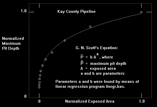
Review G. N. Scott's 1933
analysis of Kay County pipeline maximum pit depth versus
exposed area and analyze the data by linear regression.
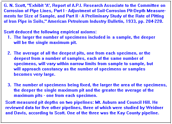
I, Glenn E. Bowie, studied G. N. Scott's 1933
analysis in 1975. My results as well as those of four
co-authors were published in a research and development
report. The reference to Scott's work is given in the
following image:


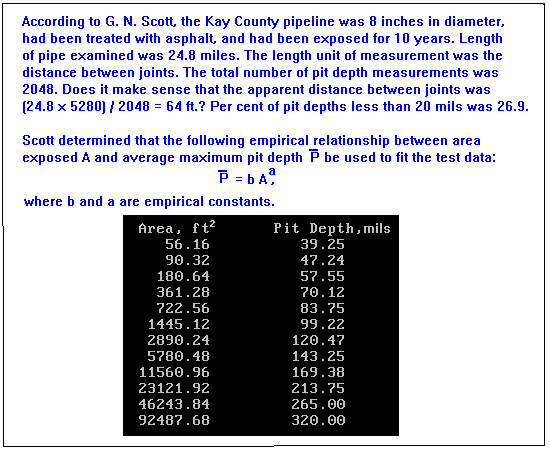
There are 12 pairs of measurements in the Kay County pipeline
data set. We need to file them. Use the QBasic icon in your
wtt02 Course I program group. Open program pairfile.bas.
Run the program, enter Kay as file name and 12 as the
number of data pairs. Enter the first pair as 56.16, 39.25
and the
remaining 11 pairs as you are prompted to do so. On exiting the
program you will have made data file Kay.dat in directory wtt02.
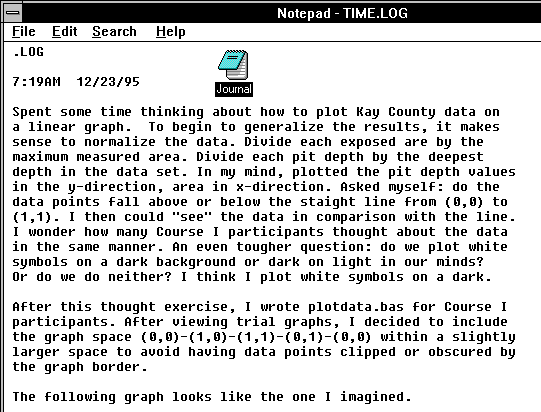
We need to think about the data set before analyzing it by means
of a linear regression program. Divide the largest area by the
smallest. Find the ratio = 1647. Now divide the deepest maximum
pit depth by the shallowest. The ratio = 8.15. Imagine a linear
graph with depth on the y-axis and area on the x-axis. Plot the
data points in your mind. You see a curve. Can you describe it?
G. N. Scott attached particular significance to the Kay County
pipeline example because it represented maximum pit depths over the
largest length of pipeline available to him and the line examined
traversed "a great variety of soil, topographical and other
conditions." See p. 206 in the above reference to Scott's report.


In 1995, I
prepared the following files to accomplish Task 1. As
a student of engineering, you have the opportunity to
duplicate the results in order to satisfy yourself
that you have met self-imposed performance-based
training objectives.
- Kay.dat --- Measured corrosion pit depths and exposed
areas
- pairfile.bas --- QBasic routine to prepare a data file
- plotdata.bas --- QBasic routine to plot normalized depth
versus area
- linrgr.bas --- QBasic routine to solve G. N. Scott's equation
and plot
In the United States, the most extensive studies of pitting corrosion
were performed at the National Bureau of Standards. Congress approved
funding for investigation of stray current electrolysis of buried
pipelines in vicinities of street railways in 1910. Field and laboratory
were carried out in the following eleven years. More general
investigations were conducted from 1922 to 1955. By the early 1930's,
the following two important empirical corrosion effects were known:
- at a given time of exposure maximum pit depth depends on
the amount of surface area inspected
- maximum pit depth for a given surface area increases relatively
rapidly in the first few years of exposure and increases less
rapidly at longer exposure times
QBasic
programs linrgr.bas, wybrgr01.bas, and wybrgr02.bas
were prepared to help you accomplish performance-based
training objectives. The following code fragment is given to
remind you to let QBasic know where you have placed data file
Kay.dat.
REM ************************************************
REM * Written by CorTech Training for WTT Course II
*
REM * linrgr.bas *
REM ************************************************
'
CLS
PRINT "ENTER FILE NAME, EX. Kay";
INPUT FILE$
FILE$ = "C:\wtt02\" + FILE$ +
".DAT"
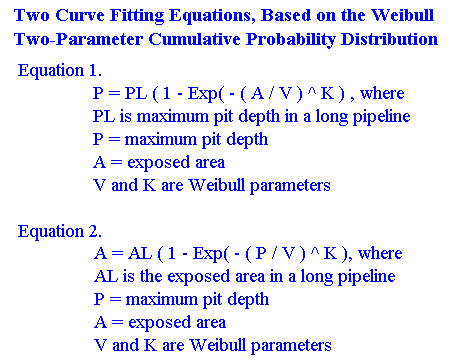
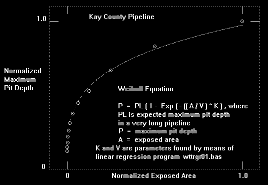
Analyze the Kay County data by
means of two Weibull curve fitting relations and compare with Scott's
results.


CorTech Training prepared the
following files for course participants:
- Kay.dat --- Measured
corrosion pit depths and exposed areas
- wttrgr01.bas --- QBasic
routine to solve the first Weibull equation, where
maximum pit depth P is regarded as a function of
exposed area
- wttrgr02.bas
--- QBasic
routine to solve the second Weibull equation, where
exposed area is regarded as a function of maximum pit
depth
Apply Weibull relations to G. N. Scott's Mt. Auburn and Council Hill
data and to Mahoning and Almeda-Lynchburg data obtained by other investigators.
In 1933, G. N. Scott published results of maximum corrosion pit depth
analyses, performed while serving as API Research Associate at the US
Bureau of Standards. His paper reveals his highly intuitive understanding of
extreme value statistics. He was vitally interested in measurement and
interpretation of maximum corrosion pit depth as a function of exposed
pipeline surface area.
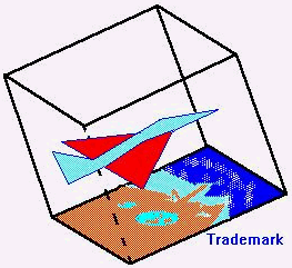
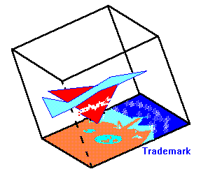
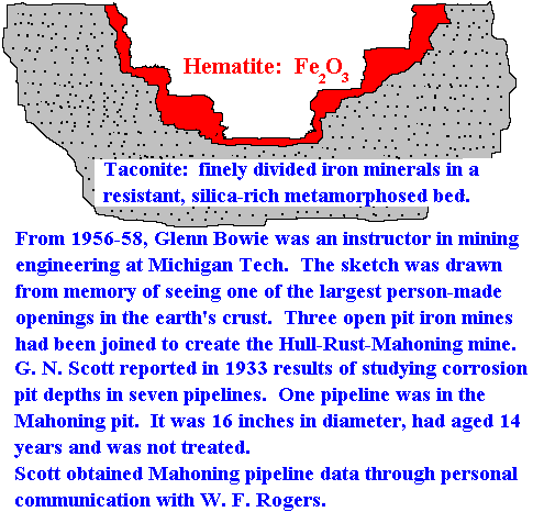
The following image reminds me of
many good times spent at Lockheed's Rye Canyon Research and
Development Center two decades ago. I had a wonderful opportunity to study
distributions of corrosion pit depth data while working at Rye Canyon.
I also think of the open pit mines I saw in Minnesota four decades ago.
Steel was made from open pit mine oxides of iron. Many of the steel
components made from the iron ore now are protected by crusts of rust,
or iron oxides with compositions similar to the parent iron ore.

In Northern Minnesota open pit mines, hematite was a direct shipping ore. It
was only necessary to scoop up relatively loosely consolidated red earth to
ship by rail to the head of Lake Superior and by freighter to hungry open
hearths at lower Great Lake ports. It was common for property owners and
mining companies to contract for removal of all the high grade ore in the pits.
Owners were paid for the amounts removed, even if local geometry of a pit
made mining relatively costly. While male miners operated machines, female
miners swept remnants of ore into baskets to ensure complete removal. The
mine openings were indeed people-made, not just man made.
Scott was involved in measuring pit depths on two of the
seven pipelines discussed in his 1933 report. The Mt. Auburn and Council Hill
pipelines were 3 years old, the first was 8 in. diameter and the second 10 in.
Mt. Auburn pipeline was treated with enamel, and Council Hill was painted thinly. Mt.
Auburn was 1024 ft. long, and measurements were made at increments of 1 ft.
Council Hill was 992 ft. long, and interval was 1 ft. It would be a very
worthwhile project for a student to determine whether Scott's 1024 Mt.
Auburn and 992 Council Hill pit depth measurements can be recovered from
US Bureau of Standards archives.
Scott reported maximum corrosion pit depths for 11
exposed areas on each of the two pipelines. For example, he reported a maximum
pit depth of 27.59 mils in the smallest of the 11 exposed areas, 2.258 sq. ft.
for the Mt. Auburn case. If we assume the pipe had an internal diameter of 8 in.
and a wall thickness of 0.125 in., then the outer diameter was 8.25 in. In that event, a
length of pipe equal to 12 in. would have an external surface exposed area of
2.258 sq. ft. This interpretation does not make sense. The wall thickness
seems insufficient. It is more likely that the wall thickness was greater than 0.3
in. Then 8 in. must have been the nominal innner diameter of a pipe with an
actual inner diameter of 8.25 in. Scott's reported exposed areas must be
internal surface areas. His sequences of exposed areas are binomial. Raise 2
to the power 10 and multiply by 2.258 to obtain 2312.192. The largest
exposed area for the Mt. Auburn case was 2312.192 sq. ft., according to
Scott. Maximum pit depth measured in 1024 ft. was 78.00 mils.
Course II includes QBasic
programs linrgr.bas, wttrgr01.bas, and wttrgr02.bas. These programs
were prepared to help you accomplish performance-based
training objectives. The following code fragment is given to
remind you to let QBasic know where you have placed data file
Auburn.dat.
REM ************************************************
REM * Written by CorTech Training for WTT Course II *
REM * linrgr.bas *
REM ************************************************
'
CLS
PRINT "ENTER FILE NAME, EX. AUBURN";
INPUT FILE$
FILE$ = "C:\wtt02\" + FILE$ +
".DAT"
CorTech Training prepared the
following files for course participants:
- auburn.dat, council.dat, mahoning.dat,
almeda.dat --- Measured corrosion pit depths and exposed areas
- wttrgr01.bas --- QBasic
routine to solve the first Weibull equation, where
maximum pit depth Px is regarded as a function of
exposed area
- wttrgr02.bas --- QBasic
routine to solve the second Weibull equation, where
exposed area is regarded as a function of maximum pit
depth
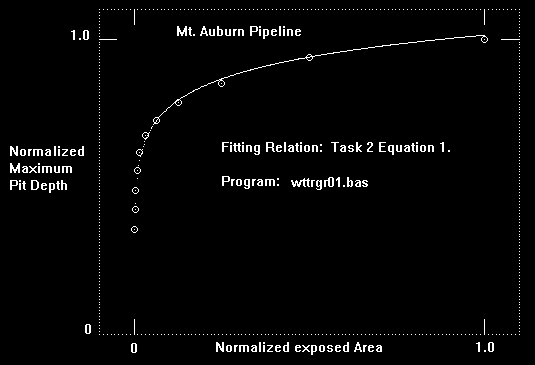
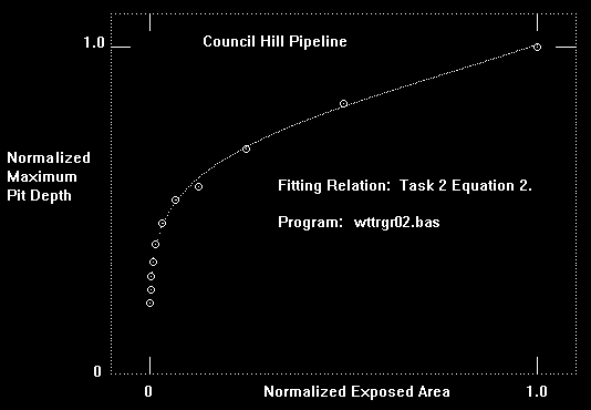
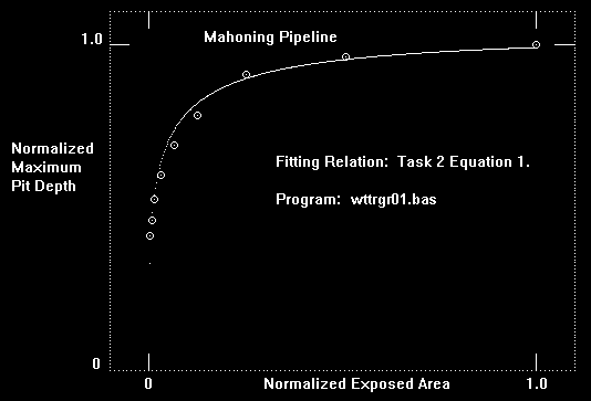
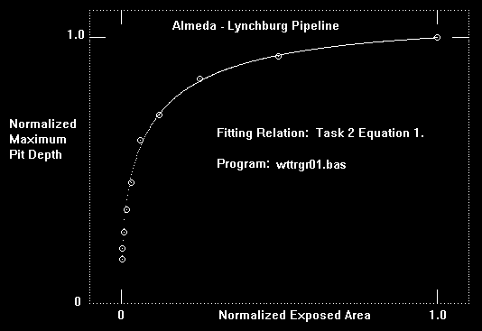
In Task 3, course participants explore applications of
two, two-parameter Weibull relations to four pipelines. The following normalized graphs
summarize one set of results.


I urge serious students of material property behavior to reproduce the
numerical and graphical results summarized in Task 4.
Review G. G. Eldrege's 1957 interpretation of Bessemer steel data
obtained by K. H. Logan(1945) and analyze the data by Weibull analyses.
In 1945, K. H. Logan presented results of tests performed on two sizes of Bessemer steel and
wrought iron specimens buried in 38 types of soils for 12 years. Ref: K. H. Logan,
Underground Corrosion, Circular of the Bureau of Standards C450, Bureau of Standards, US
Department of Commerce, 1945. On 11/29/95, the author of this course received an e-mail
message from Didier Crusset, ANDRA, France, concerning Circular 579, dated 1957, by M.
Romanoff with the same title as Logan's Circular C450. In his message, Didier stated he is
interested in clay soils with steel specimens and in analysis of general and pitting
corrosion.
In March 1957, three papers were presented at a corrosion engineers' conference on
application of extreme value statistics to interpretation of pit depth data. Papers by G. G.
Eldredge and P. M. Aziz were published subsequently. A paper by G. N. Scott was
presented but not published. It is probable that the three authors were influenced by a report
by E. J. Gumbel: Statistical Theory of Extreme Values and Some Practical Applications, US
Bureau of Standards, Applied Mathematics Series No. 33, 1954.
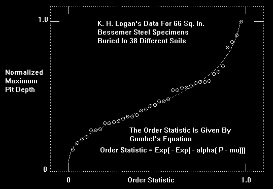
G. G. Eldredge applied Gumbel's double exponential function to interpretation of K. H.
Logan's data. Eldredge used the equation
F(Px) = Exp(- Exp( - alpha(Px - mu))),
where Px is maximum pit depth in a specimen and alpha and mu are parameters of the
distribution.
After Gumbel, Eldredge approximated F(Px) by means of the order statistic i /(N +
1), where i is the rank order of a specimen with maximum pit depth Px(i) and N equals the
number of soil types, 38. Eldredge found values of alpha and mu by graphical techniques.
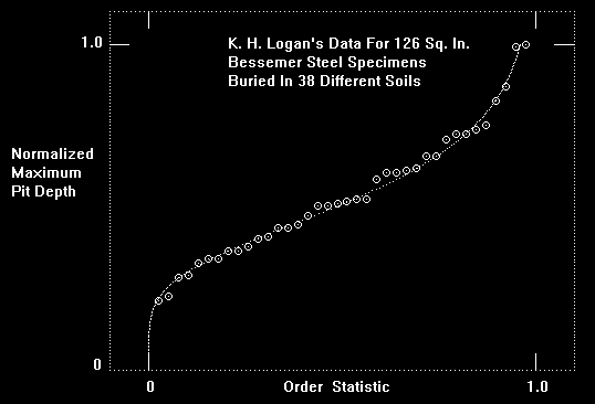
For this course there are two Bessemer steel specimen data files, bess66.dat and bess126.dat,
each containing 38 maximum pit depths rank ordered from smallest to largest. File bess66.dat
contains Logan's data for 66 sq.in. Bessemer steel specimens and bess126.dat the 126 sq. in.
specimen data. Program gumrgr.bas was written for those course participants who actually
perform suggested exercises. The program
can help you determine parameters alpha and mu for the two data sets. The following two
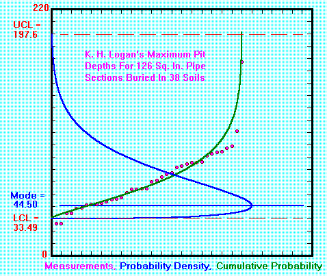
graphs show how well Gumbel's double exponential distribution applies to interpretation of
Logan's data.


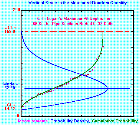
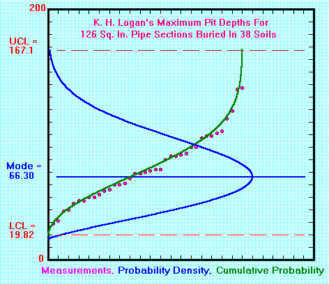
Weibull Trending Toolkit
Three executable programs in the Weibull Trending Toolkit find three parameters of the
Weibull distribution by the method of moments. A program matches sample and Weibull
mean, standard deviation, and skewness in the process of finding three Weibull parameters k,
e, and v. The Weibull distribution for maximum pit depths Px may be expressed as
F(Px) = 1 - Exp(-((Px - e)/(v - e))^k), where
parameter e is the Weibull threshold value, v is the characteristic value, and k is the Weibull
exponent. In present form, the Weibull Trending Toolkit applies only to cases where exponent
k is greater than 1.0. When k is greater than 1.0, the distribution has a most frequent value.
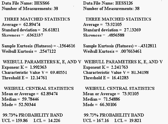
The most frequent value is called the mode. Program wtutor.exe was applied to data files
bess66 and bess126 to obtain results shown below. Pit depths are in units of mils. Specimen
areas were 66 sq. in. and 126 sq.in.


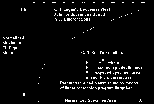
Course participants may use Weibull modal maximum pit depth values and the two specimen
areas to write data file bessemer.dat. Two pairs of values may be analyzed by means of Task
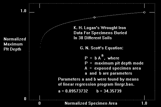
1 program linrgr.bas to estimate parameters a and b in Scott's power law equation.

CorTech Training prepared the following files for participants:
- bess66.dat, bess126.dat, and bessemer.dat
- gumrgr.bas --- QBasic routine to find Gumbel distribution parameters
- wtt01.exe --- executable program to find three parameters of the
Weibull distribution
Every trainer takes her
or his own course. I took this course by preparing it. The first
time was in 1975, the second in 1996. It takes a lot of detailed,
individual effort to extract meanings from historic pit depth
data sets. There is satisfaction in finding simple relations
which can model the data. By understanding past material corrosion
behavior we can better predict future behavior.
Analyze K. H. Logan's
1945 wrought iron specimen data and compare with Bessemer
steel specimen results.
In 1945, K. H. Logan
presented results of tests performed on two sizes of Bessemer
steel and wrought iron specimens buried in 38 types of soils
for 12 years. Ref: K. H. Logan, Underground Corrosion,
Circular of the Bureau of Standards C450, Bureau of
Standards, US Department of Commerce, 1945.
were presented at a corrosion engineers' conference on
application of extreme value statistics to interpretation of
pit depth data. Papers by G. G. Eldredge and P. M. Aziz were
published subsequently. A paper by G. N. Scott was presented
but not published. It is probable that the three authors were
influenced by a report by E. J. Gumbel: Statistical Theory of
Extreme Values and Some Practical Applications, US Bureau of
Standards, Applied Mathematics Series No. 33, 1954.
Eldredge applied Gumbel's double exponential function to
interpretation of K. H. Logan's data. Eldredge used the
equation F(Px) = Exp(-(-alpha(Px - mu))), where Px is maximum
pit depth in a specimen and alpha and mu are parameters of
the distribution.
After Gumbel, Eldredge approximated F(Px) by means of the
order statistic i/(N + 1), where i is the rank order of a
specimen with maximum pit depth Px(i) and N equals the number
of soil types, 38. Eldredge found values of alpha and mu by
graphical techniques.
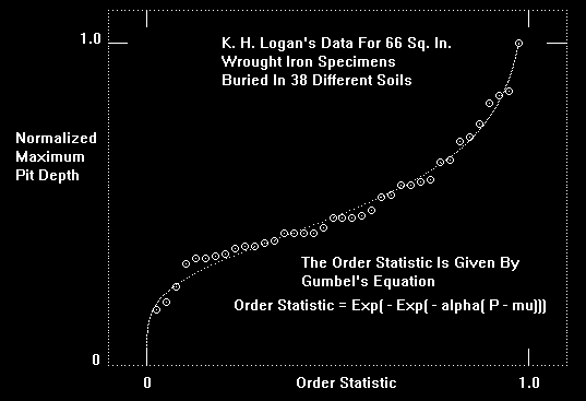
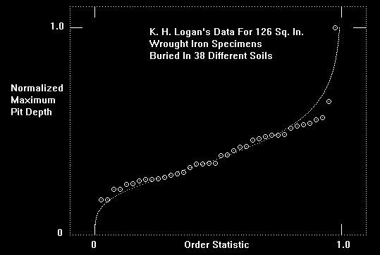
For this course there are
two wrought iron specimen data files, wfe66.dat and
wfe126.dat, each containing 38 maximum pit depths rank
ordered from smallest to largest. File wfe66.dat contains
Logan's data for 66 sq.in. wrought iron specimens and
wfe126.dat the 126 sq. in. specimen data. Program gumrgr.bas
was written for course participants to determine parameters
alpha and mu for the two data sets. The following two graphs
show how well Gumbel's double exponential distribution
applies to interpretation of Logan's data.
 
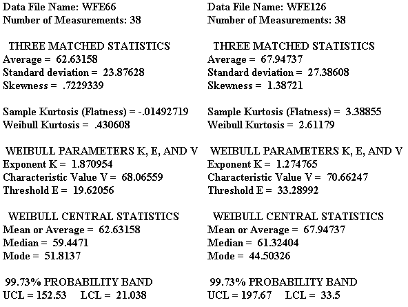
Weibull
Trending Toolkit
Three executable programs
in the Weibull Trending Toolkit find three parameters of the
Weibull distribution by the method of moments. A program
matches sample and Weibull mean, standard deviation, and
skewness in the process of finding three Weibull parameters
k, e, and v. The Weibull distribution for maximum pit depths
Px may be expressed as
F(Px) = 1 -
Exp(-((Px - e)/(v - e))^k), where
parameter e is the Weibull
threshold value, v is the characteristic value, and k is the
Weibull exponent. In present form, the Weibull Trending
Toolkit applies only to cases where exponent k is greater
than 1.0. When k is greater than 1.0, the distribution has a
most frequent value. The most frequent value is called the
mode. Program wtutor.exe was applied to data files wfe66 and
wfe126 to obtain results shown below. Pit depths are in units
of mils. Specimen areas were 66 sq. in. and 126 sq.in.
Weibull
Numerical and Graphical Results


In Task 4, Weibull modal
maximum pit depth values and the two specimen areas were used
to write data file bessemer.dat. Two pairs of values were
analyzed by means of Task 1 program linrgr.bas to estimate
parameters a and b in Scott's power law equation. As can be
seen above, the Weibull modal estimate for 66 sq. in. wrought
iron specimens is 51.81 mils and for 126 sq. in. specimens
the estimate is 44.50 mils. Scott did not anticipate a
decrease in modal depth with increase in specimen area.
However, the Gumbel analyses for wrought iron specimens
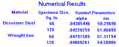
yielded different modal estimates. The parameter mu in
Gumbel's equation is an estimate of modal value. For 66 sq.
in. specimens the Gumbel mode equals 50.29696 mils and the
126 sq. in. specimen mode equals 61.06899 mils. MS-DOS editor
Edit was used to write file wrought.dat and QBasic was used
to run program linrgr.bas to obtain the following result.


Modeling
Weibull Behavior
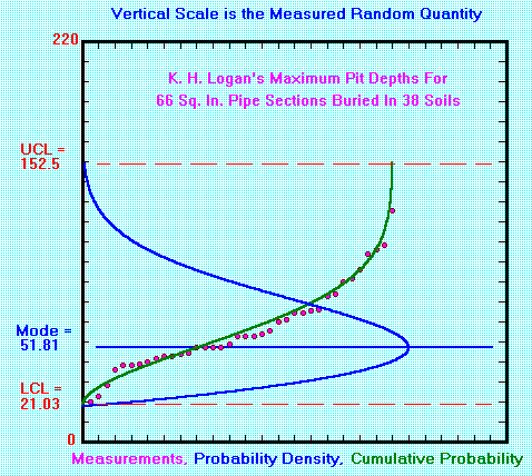
All four Weibull
probability density distributions are positively skewed. The
distributions have relatively long tails toward deeper
maximum pit depths. The Weibull exponent k for 126 sq. in.
wrought iron specimens seems to be significantly lower than
the exponents for the other three cases. There is a
possibility that surficial material properties of 126 sq. in.
wrought iron specimens were different than those of the 66
sq. in. specimens. Seemingly exceptional numerical results do
not necessarily imply that experimental results are not in
order.
The average of three
Weibull exponents equals 2.035. The average of four threshold
values equals 20.37 mils and the average of four
characteristic values equals 70.37 mils. All of Logan's
maximum pit depth measurements for two iron based alloys and
two specimen sizes may be modelled by means of the Weibull
cumulative distribution
F(Px) = 1.0 -
Exp(-((Px - 20)/(70 - 50)^2)
If, for example, it is
desired to model the upper control limit at 100 x F(Px) =
98.865% then
UCL = 20 +
50(-LOG(1 - 0.99865))^(1/2) = 149 mils.
A more conservative model
could be chosen by letting k = 2, v = 70, and e = 0. In that
event the model is a Rayleigh distribution
F(Px) = 1.0 -
Exp(-(Px/70)^2)
For this model, 99.865% of
the maximum pit depths would be predicted to be less 180
mils.
Comparison
Of Weibull And Gumbel Results For Bessemer Steel And Wrought
Iron Specimens
In his 1957 review of K. H.
Logan's 1945 data, G. G. Eldredge decided the effect of
difference in specimen size could be accounted for on extreme
value probability graphs by shifting a linear fitting
relation by an amount equal to the logarithm of the specimen
area ratio. He concluded that differences in maximum pit
depths for the Bessemer steel specimens could be accounted
for in terms of an area effect, but pit depth differences for
the wrought iron specimens could not. WTT Course I
participants are encouraged to discuss the Bessemer steel and
wrought iron specimen results.
Task 6 is the first of four Tasks about pitting corrosion in
aluminum alloys. The first experimental data set analyzed
includes effects of time of exposure. I suggest you follow
the Tasks meticulously. If you are a student, retiree, or
particularly diligent working technician or engineer, try to
repeat the steps taken to deduce curve fitting relations,
tables, and graphs.
Review P. M. Aziz's 1956
experimental procedures and data
for Al alloy specimens immersed in Kingston tap water

P. M. Aziz, "Application of the Statistical Theory of
Extreme Values to the Analysis of Maximum Pit Depth Data for
Aluminum", Corrosion, Vol. 12, October 1956, pp.35-46.
Aziz described experimental procedure on pp. 38-39:
"Strings of 2S-O alloy sheet, ten panels to string,
were prepared by threading 5 inch x 2 inch coupons on glass
hangers through 3/8 inch holes centered 3/4 inch from the top
of the panels. These were vapor degreased using
trichloroethylene, etched for two minutes in 85 percent
phosphoric acid at 70 deg. C and washed for half an hour in
cold running water; they were then immersed in a 300 gallon
tank of Kingston tap water, held at 25 deg. C. The water
flowed continuously and slowly and changed every 24 hours.
The immersion periods ranged from one week to one year.
At the end of each time period a string was removed from
the tank, cleaned of corrosion products and the depth of all
the pits on both sides of each of the ten panels measured by
the calibrated microscope technique. These data were grouped
over the pit depth ranges 0-99, 100-199 microns etc., and
frequency curves were constructed for the various time
periods."
Aziz interpreted his frequency distribution curves as having
J-shaped and bell-shaped portions. Aziz estimated modal pit
depths for the bell-shaped portions and compared modes a as a
function of exposure time. He found the mode apparently
stabilized after exposure for two months. He noted the maximum
pit depth in a data set for exposure times greater than two
months continued to increase even though the mode had stabilized.
On p. 45 of his paper he concluded:
- When freshly etched aluminum is immersed in an
aggressive water a relatively large number of pits
initiate and develop to the stage where they become
visible.
- Within two weeks more than half of the pits that
start stifle themselves and become inactive. A pit
depth distribution curve for this group takes the
form of the letter J with many very shallow pits and
a few that go somewhat deeper.
- The remaining pits continue to propagate for about
two months. A pit depth distribution curve for this
group has the familiar bell shape. During this period
all pits propagate at about the same rate and the
"bell" type curve retains its shape and
moves in the direction of increasing depth.
- After about two months the majority of these pits
become stifled and only a small number of the deeper
ones continue to propagate. Thus the bell shaped
curve remains stationary but develops a tail that
lengthens with time.
It is probable that P. M. Aziz was influenced by a report by
E. J. Gumbel: Statistical Theory of Extreme Values and Some
Practical Applications, US Bureau of Standards, Applied
Mathematics Series No. 33, 1954.
Aziz applied Gumbel's double exponential
function to interpret the aluminum specimen data. He used the
equation
F(Px) = Exp(-(-alpha(Px - mu))),
where P is maximum pit depth in a specimen and alpha and mu are
parameters of the distribution.
After Gumbel, Aziz approximated F(Px) by means of the order
statistic i/(N + 1), where i is the rank order of a specimen with
maximum pit depth Px(i) and N equals the number of number of
specimens in a string, that is ten specimens. He found values of
alpha and mu by graphical techniques.
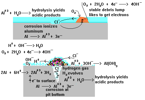
Those course participants who learn by doing are encouraged to
discuss Aziz's description of shallow pits which stifle
themselves and deeper pits which continue to grow in a stable
manner. The sketches at page top were included to assist
discussion.
Data Obtained By P. M. Aziz, 1956

Task 7 is the second of four Tasks about pitting corrosion in
aluminum alloys. The first experimental data set analyzed
includes effects of time of exposure. I suggest you follow
the Tasks meticulously. If you are a student, retiree, or
particularly diligent working technician or engineer, try to
repeat the steps taken to deduce curve fitting relations,
tables, and graphs.
Interpret Aziz's pit depth frequency
distributions by Weibull analysis.
P. M. Aziz, "Application of the Statistical Theory of
Extreme Values to the Analysis of Maximum Pit Depth Data for
Aluminum", Corrosion, Vol. 12, October 1956, pp.35-46.
- Download the completely free self-extracting Weibull Trending
Toolkit wtt01.exe from an archive.
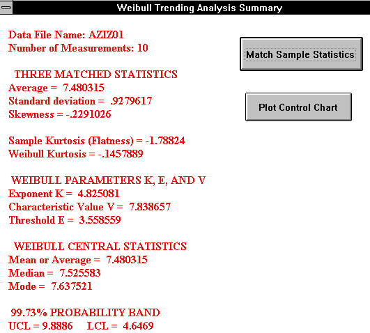
- Use QBasic program makefile.bas to make data file aziz01.dat for the specimens exposed for
one week. Convert pit depth units from microns to mils.
Run program wrisk.exe, which is included it archive wtt02.exe.

- Study three-parameter Weibull analysis results.

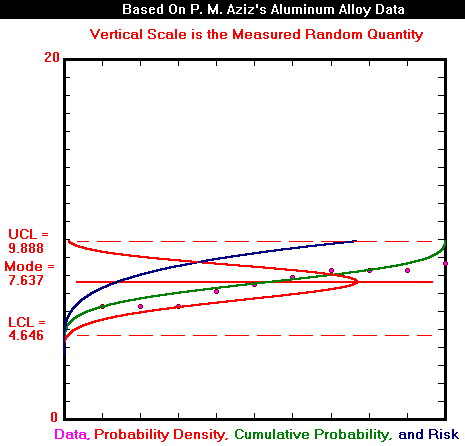
- With the one year data in mind, select a graph upper
limit of 20 mils. Study the resulting Weibull curves.

Task 8 is the third of four Tasks about pitting corrosion in
aluminum alloys. The first experimental data set analyzed
includes effects of time of exposure. I suggest you follow
the Tasks meticulously. If you are a student, retiree, or
particularly diligent working technician or engineer, try to
repeat the steps taken to deduce curve fitting relations,
tables, and graphs.
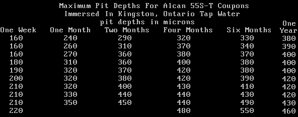
Interpret Aziz's Alcan 55S-T
maximum pit depth data for either 9 or 10 specimens at each of
six exposure times.
P. M. Aziz, "Application of the
Statistical Theory of Extreme Values to the Analysis of Maximum
Pit Depth Data for Aluminum", Corrosion, Vol. 12, October
1956, pp.35-46.
- Make data files aziz01.dat through
aziz06.dat for the specimens exposed for six exposure
times. Convert pit depth units from microns to mils. Run
program wrisk.exe. Study three-parameter Weibull analysis
results.


Task 9 is the last of four Tasks about pitting corrosion in
aluminum alloys. The first experimental data set analyzed
includes effects of time of exposure. I suggest you follow
the Tasks meticulously. If you are a student, retiree, or
particularly diligent working technician or engineer, try to
repeat the steps taken to deduce curve fitting relations,
tables, and graphs.
Generalize interpretation of
Aziz's data to obtain a relation in terms of exposed area,
maximum pit depth, and exposure time.
Programs WRISK.EXE and WDESIGN.EXE used in Task 9 were prepared in 1996. They each contain a
first screen which is to be ignored. An e-mail address given there is obsolete.
References
- P. M. Aziz, "Application of the
Statistical Theory of Extreme Values to the Analysis
of Maximum Pit Depth Data for Aluminum",
Corrosion, Vol. 12, October 1956, pp.35-46.
- H. P. Godard, W. B. Jepson, M. R.
Bothwell, and R. L. Kane, "The Corrosion of
Light Metals", John Wiley and Sons, Inc., New
York, 1967.
Analysis
P. M. Aziz's Data
Task 8 Suggestions
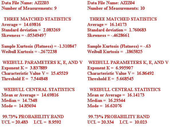
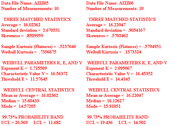
- Make data files aziz01.dat through aziz06.dat for the
specimens exposed for six exposure times.
- Convert pit depth units from microns to mils.
- Run program wrisk.exe. Study three-parameter Weibull
analysis results.
Task 9 Suggestions
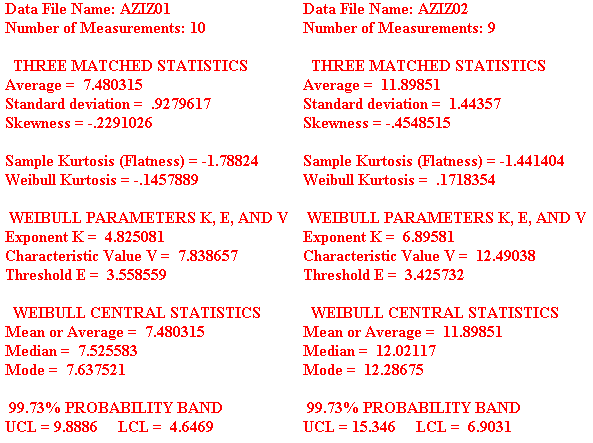
- Examine results in Task 8 in pairs. Average Weibull
threshold parameter E for exposure times of one week and
one month equals 3.49 mils. Average E for exposure times
of six months and one year equals 13.0 mils. Average
Weibull characteristic value V also increased with
exposure time. The Weibull shape parameter K seems to
have a random behavior. It is clear that some smoothing
or grouping of Aziz's data must be used to generalize
shape parameter behavior.
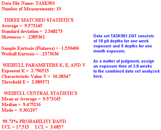
- Group Aziz's data for exposure times of one week and one
month into data file task901.dat using MS-DOS Edit.
Express the 19 values in units of mils.
- Group Aziz's data for the remaining four exposure times
into a set of 39 maximum of depths, mils, in file
task902.dat.
- Apply QBasic program SORT.BAS given in the Weibull
Trending Toolkit to files task901.dat and task902.dat.
SORT does just that, and creates two new files
otask901.dat and otask902.dat.
- Apply Weibull Trending Toolkit program WRISK.EXE to files
otask901 and otask902. Program sees the leading o's and
calls the sorted files TASK901 and TASK902.
- Examine WRISK numerical results for files task901 and
task902.
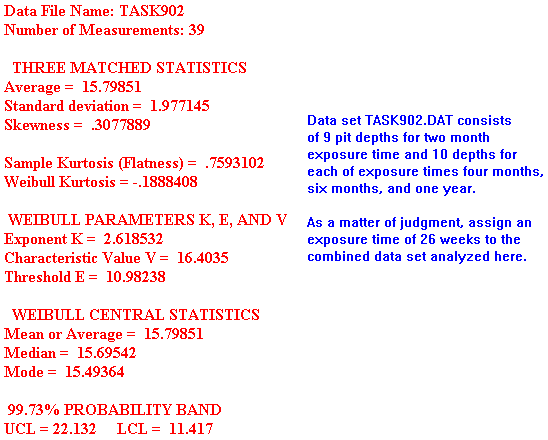
Numerical Results for 19 Maximum Pit Depths

Numerical Results for 39 Maximum Pit Depths

Plot Grouped Data
Use WRISK to plot results for data files task901 and
task902 with graph upper limit equal to 30 mils in each
case.
Superimpose the two graphs to obtain the following image.

Include H. P. Godard's Industrial Water Pipeline Data
- Examine H. P. Godard's industrial water pipeline data on
p. 64 of the above reference. He measured maximum pit
depth in each of 20 three foot long sections of AA 5052
pipe after 13 years exposure.
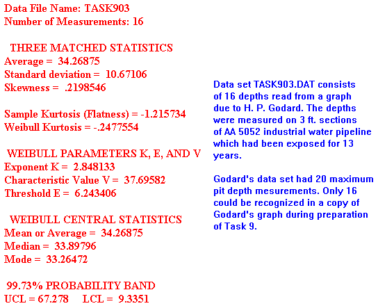
- The instructor was able to read 16 pit depths from
Godard's graph. As a course participant, you may make data
file task903.dat to store Godard's data.
- Apply program WRISK to file task903.
- Examine the following numerical results.

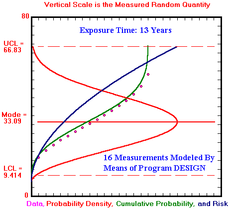
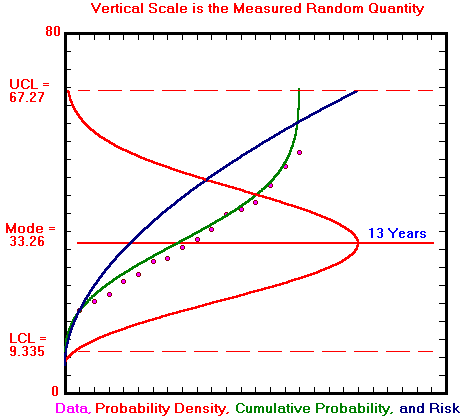
- Plot results of analyzing Godard's data. Choose a graph
upper limit of 80 mils.

Create Modeling Program DESIGN
- Notice the Weibull shape parameter K values for files
task901, task902, and task903
have much less variation than the K values for data files studied
in Task 8.
- Average the three K values found here to obtain K = 2.75439.
- After some thought, decide to use E and V values for files
task901 and task903 to
model time dependence. Let E = A * T + B and V = C * T + D, where
T is exposure time
in years and A, B, C, and D are constants.
- The Weibull Trending Toolkit includes a program called
WDESIGN. It uses an order statistic to estimate N probabilities.
A user supplies
trial Weibull exponent K, threshold E and an estimate of the
median random variable.
The program estimates N values of the variate and finds Weibull
K, E, and V to
match design sample and Weibull mean, standard deviation, and
skewness, values.
- The instructor used WDESIGN as the basis for creating new
program DESIGN.
- DESIGN has an exponent K which is independent of exposure
time,
and parameters
E and V which are linearly dependent on time exposure. When a
user runs DESIGN,
she/he is prompted to input a file name, number of measurements N
being modeled,
and exposure time.
- DESIGN uses an order statistic base on N, the constant K, and
calculated E and V
to generate N design sample maximum pit depths.
- DESIGN matches sample and Weibull mean, standard deviation,
and skewness
values to find K, E, and V
for the N design measurements.
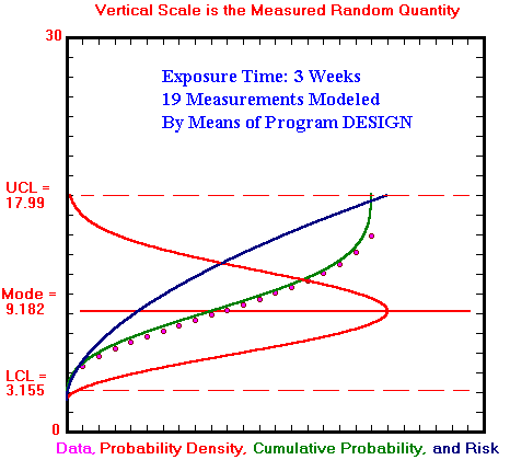
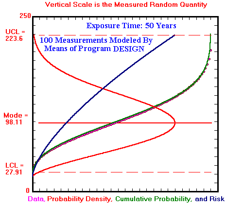
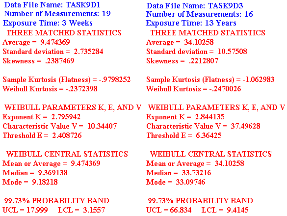
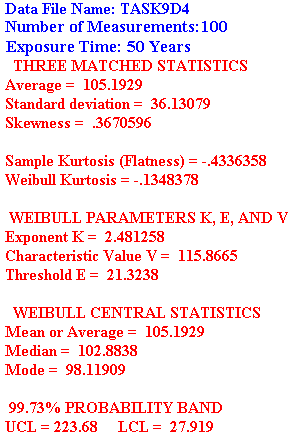
Model Grouped Aziz Data for Three Week
Exposure and Godard Data for 13 Year Exposure

 
Industrial Water Pipeline with 50 Year
Design Life


Note written in 1995 about using wrisk.exe and risk.bas.
The Weibull Trending Toolkit Program wrisk.exe is 1995
copyrighted property of:
Glenn E. Bowie
2426 Hallquist Ave.
Red Wing, MN 55066
(651) 388-2374
e-mail: glennbowie@hotmail.com

Do not try to use WRISK.EXE to process a file with more than 1024
data values.  WRISK.EXE runs on an IBM compatible PC with Microsoft
Windows.  Make sure you have VBRUN300.DLL in your
C:\>WINDOWS\SYSTEM directory.


The Weibull Trending Toolkit program WRISK.EXE has three curves instead
of two.
blue = Weibull probability density
green = Weibull cumulative probability
yellow = Weibull risk
Weibull Probability Density, p

p = k * ((x - e)/(v - e)^(k - 1) *

Exp(-((x - e)/(v - e))^k/(v - e).

Weibull Cumulative Probability, F

F = 1 - Exp(-((x - e)/(v - e))^k)

Let P = Exp(-((x - e)/(v - e))^k)

Weibull Risk

R = k * ((x - e)/(v - e))^(k - 1)/(v - e)

You see that p = R * P, or R = p/P.

The probability density and risk curves are scaled so you can see their
shapes.  When you are ready to study probability density and risk mag
nitudes, you can use QBasic program RISK.BAS as a starting tool.

I like to use to PCs side by side when studying Weibull risk.  A good
starting point is to examine file 6061.DAT using Edit.  There are 102
fatigue lives in the file.  The first two lives are 233 and 258.  Count
down to find the median life in the file equals 400.  Examine the last
entry in the file.  The 102nd value in the file is 560.

Run WRISK and choose file 6061.  Use a graph upper limit = 800.
There are 19 tics on the Y-axis.  Each scale division is worth 40 life
units.  20 x 40 = 800.  From the summary screen,
k = 3.61498
e = 195.1232
v = 420.0841
Median = 398.3941

Type QBasic risk, press enter on your second PC.  RISK asks you for
the Weibull shape parameter k, threshold parameter e, median, and
production run size.  Enter the above values for k, e, and median and
102 for production run size.  RISK tells you characteristic value v =
420.0842.  The value in the summary screen of WRISK is truncated
rather than rounded.  We accept that the two characteristic values
are the same.  RISK tells you the probability of survival at the first
failure is 0.9903.  The cumulative distribution curve, green, is a
probability of failure curve.

P = probability of survival
F = probability of failure
F = 1 - P.

The height of the green curve is 1 - 0.9903 or 0.0097 at the first
failure, according to RISK.  RISK predicts the time to first
failure = 257.6.
Compare with actual first experimental value in 6061.DAT, 233.  RISK
tells us the probability density at time 257.6 equals 0.0005588.
Calculate the risk at first failure:

R = p/P = 0.0005588/0.9903 = 0.0005643.  RISK tells us
R = 0.0005643 at first failure.

Work your way through second failure comparisons at your leisure.
Move to the median.  RISK predicts the median life equals 398.3941,
and the experimental value is 400.  WRISK shows the mean, median,
and mode are close together for file 6061.  RISK tells us the height of
the probability density curve at the median equals 0.00616.  And at time
538.956, the density drops back down to 0.000473.  The difference in
time units between the last failure and the threshold e equals 538.956 -
195.1232 = 343.8328.  Multiply this difference by the density at the
median to obtain 2.1192.  Remember the area of a triangle equals 0.5 x
base x height.  We just estimated the area under the density curve to be
0.5 x 2.1192 = 1.0596.  The area under a probability density curve
equals 1.0.

I used a clear, plastic scale divided in mm to find the height of the
yellow risk curve at the mode and at 538 time units to be 19 and 79 mm.
The height ratio equals 19/79 or 0.24.  RISK predicts the ratio to be
0.0123/0.0487 = 0.25.

Stare at the graph for file 6061.  Use a scale to confirm that the
cumula tive probability is at 0.5 of the maximum height, for this case.
The probability of survival at the median = 0.5.  RISK tells us risk
R = 0.1232696 at the median.  At the median, find R x P = 0.0616348.
The density p at the median is then 0.0616348, as RISK told us already.
It is important to practice looking at the curves when interpreting
numerical results.

Look at the probability density and cumulative probability curves for
file 6061.  Think of the probability density as the rate of change of
the cumulative probability.  The slope of the cumulative probability
curve, the green one, is maximal at the mode.  The probability density
is maximal at the mode.

Glenn E. Bowie
Red Wing, MN
September 1, 1995
Note written in 1995 about using programs wdesign.exe and wrisk.exe.
The Weibull Trending Toolkit Program wdesign.exe is 1995 copyrighted
property of:
Glenn E. Bowie
2426 Hallquist Ave.
Red Wing, MN 55066
(651) 388-2374
e-mail: glennbowie@hotmail.com

It is important to remember that WDESIGN writes a data file and a
results file each time it is used.  When WDESIGN asks you for a file
name, NEVER give it the same name as an experimental file such as
6061, 7075 and so on.  It is a good practice to use the leading
letter D in all file names you give WDESIGN.  Avoid
naming experimental data files with a leading D.

Let me assume you have applied WRISK.EXE to study data file 6061 as
outlined in the above note about WRISK.  Run WDESIGN.  Click the box
"Enter N, k, e and Median".  Be sure to enter a file name.  This
time enter D6061.  Enter the following values:
For N: 102
For k: 3.61498
For e: 195.1232
For Median: 398.3941

Compare the summary results and graph with the summary and graph
you get when you apply WRISK to file 6061.  Keep the median at
398.3941 and decrease k gradually.  At each step, compare with
WRISK and 6061 results.  Finally, choose
N: 102
k: 3.55
e: 194
Median: 398.3941


Apply WRISK to file D6061.  You get the same results given by
WDESIGN for the above parameters.

Please do not apply WDESIGN for N > 1024.

Please supply design threshold e values that are sufficiently
large to keep resulting threshold values in the summary screen
positive.

Please be aware there is room for research.

Please be aware as you practice using WDESIGN in relation to your
database that you are thinking about possible application of
WDESIGN concepts for preparation of production run specifications.
___________________________________________________________________
Design Practice

At the DOS prompt, type QBasic risk.  Run RISK.BAS.  Enter shape
parameter k equal to 1, threshold parameter 0 and median 300.
See the characteristic value v = 432.8085.  Enter run size 500.
It is important to see that risk h(t) is constant from the first
to the last failure. Here h(t) = 0.002310491.  Now find 1/v.
For k = 1 and e = 0, h(t) = 1/v.  The failure rate is constant.

Many reliability and risk analysts limit their work to the special
case where the risk or failure rate is constant.  Programs
WTT01.EXE, WRISK.EXE, and WDESIGN.EXE do not apply to the special
case where k = 1.  In order to show you the difference between the
constant risk case and one where k is slightly greater than 1.0,
the following exercise was constructed.

At the DOS prompt for directory wtt02, load Windows.
C:\wtt02\win.  Hopefully, you see the Program Manager high-
lighted.  Click File, then click Run.  In the Run Window, enter
on the command line: c:\wtt02\wrisk.exe.  Click OK on the WRISK
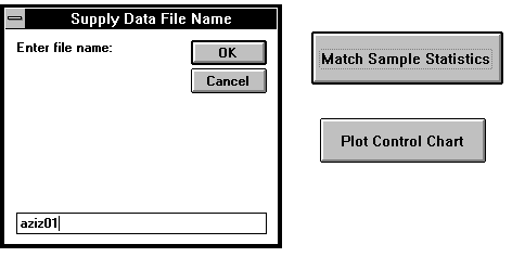
sign-on screen.  Click "Match Sample Statistics".  Enter file
name 6061.  Click "Plot Control Chart" and enter graph upper
limit 800.  You see the graph.  Notice a portion of the summary
screen is visible below the graph.  Hopefully, you also can see
the Program or File Manager word File. Click File.  Click Run.  Enter
on the command line: c:\wtt02\wdesign.exe.  Click OK on the WDESIGN
sign-on screen.  Click "Enter N, K, E, And Median".  Enter file
name delight.  For N, 500.  For K, 0.95.  For E, 27.0.
For Median, 300.

Notice k = 1.032018, and e = 0.4963179.  If you ever analyze material
property data and obtain a k value as close to 1.0 as this, with e
not negative, consider sending me a copy of your data.  See
UCL = 2743.9.
Click "Plot Control Chart" and enter graph upper limit 3000.  Examine
the yellow RISK curve.  It is a delight.  I believe risk curves such
as this one can represent many data sets which are now represented
by a constant failure rate approach.

In the lower left corner of the screen, click the small rectangular
portion of WRISK summary screen.  Click "Match Sample Statistics".
Enter file name delight.  WDESIGN generated file delight.dat.  WRISK
has now analyzed the file and obtained familiar results.  Click
"Plot Control Chart", and enter 3000.  The graph is again a delight.

Click the small rectangular portion of WDESIGN summary screen in the
lower right corner of your display.  Enter the following:
design11
500
1.1
25
300
Study the summary values.  Since UCL = 2042.8, choose graph upper
limit 2500.  Notice the risk curve.  Click anywhere on the portion
of WDESIGN summary screen visible below the graph.
Enter:
design12
500
1.2
25
300
Study the summary values.  Choose graph upper limit 2000.
Click WDESIGN summary screen at the bottom, enter:
design13
500
1.3
25
300
Choose graph upper limit 2000.  Proceed to generate file design14 with
k = 1.4, design15 with k= 1.5, and so on until you have generated file
design19 with k = 1.9.  Choose graph upper limit 1000.  It is time to
generate a particular case.
Enter file name drayly, with N = 500, k = 1.928, e = 7.9 and median
= 300.  Notice k = 1.999 and e = 0.01767976.  Choose upper limit
1000.  Describe the risk curve.
In the special case where k = 2.0 and e = 0, the Weibull distribution
becomes a Rayleigh distribution.  For a Rayleigh distribution, the risk
is a straight line.
Generate files design20, design21 and so on until you have generated
file design40.  Examine the graphs with upper limit 1000 in each case.
Watch changes in risk.
Click the portion of WRISK summary screen at lower left and review
files delight, design11 through design19, drayly, and design20 through
design40.
Examine skewness aand kurtosis values during your review.  Decide for
yourself what range of k yields probability density curves which might
be considered to be symmetrical or pseudo-normal.


Glenn E. Bowie
Red Wing, MN
September 1, 1995
 
Copyright
Glenn E. Bowie©,
CorTech Training, Red Wing, MN 1996, 2000, 2001, 2003. All rights reserved.
|
 CorTech
Training, Red Wing, MN